AP Physics 2 Unit 10 Lab

Elisa Alvarado, Sarah Cratem, Ryan Partain, Julia Reidy

Mr. Thomas

AP Physics 2 cmod

14 March 2016

Unit 10: Quantum Model Lab Report

Objective: To determine the relationship between brightness and density of light related to the current it produces.

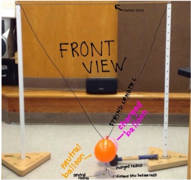
Apparatus:

Procedure:

Finding the Relationship Between Current and Photon Density
1. Choose Sodium as the target metal
2. Set the voltage to a constant 1 V
3. Set the wavelength to 250 nm
4. Set the photon density = 0.01
5. Hit “Record Data Point”
6. Change the photon density by adding 0.10. Hit “Record Data Point”
7. Repeat step 6 for (0.10,1.00]; you should have 11 data points

Finding the Relationship between Current and a Change in Potential
1. Using Sodium, set the photon density = 1
2. Set the wavelength at 250 nm
3. Set the voltage = 0 V
4. Hit “Record Data Point”
5. Change the voltage by adding 0.500V. Hit “Record Data Point”
6. Repeat Step 5 for (0.500V, 5.000V]; you should have 11 data points

Finding the Relationship between Maximum Kinetic Energy and Frequency
1. Using Sodium, set the photon density = 1, and set the voltage = 1 V
2. Start with wavelength = 800 nm; this will result in a frequency of 3.75 x1014Hz
3. Hit “Record Data Point”
4. Subtract 86 nm from the wavelength to increase the frequency. Hit “Record Data Point”
5. Repeat Step 4 for [200 nm, 700 nm)
6. Calculate by using a spreadsheet software and the equation 𝜙 (multiply Plank’s constant, eV·s, by the frequency column and subtract the work function for Sodium which equals 2.28eV)

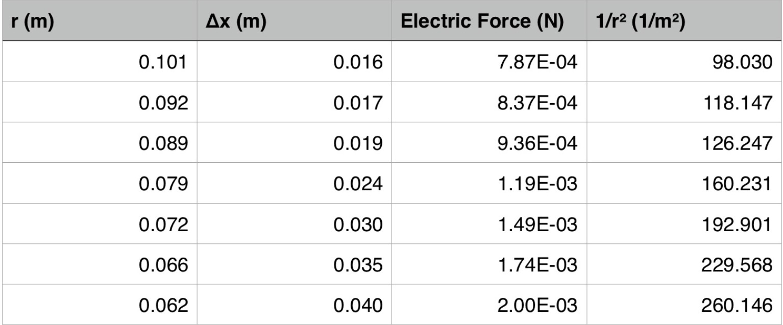
Data Table:

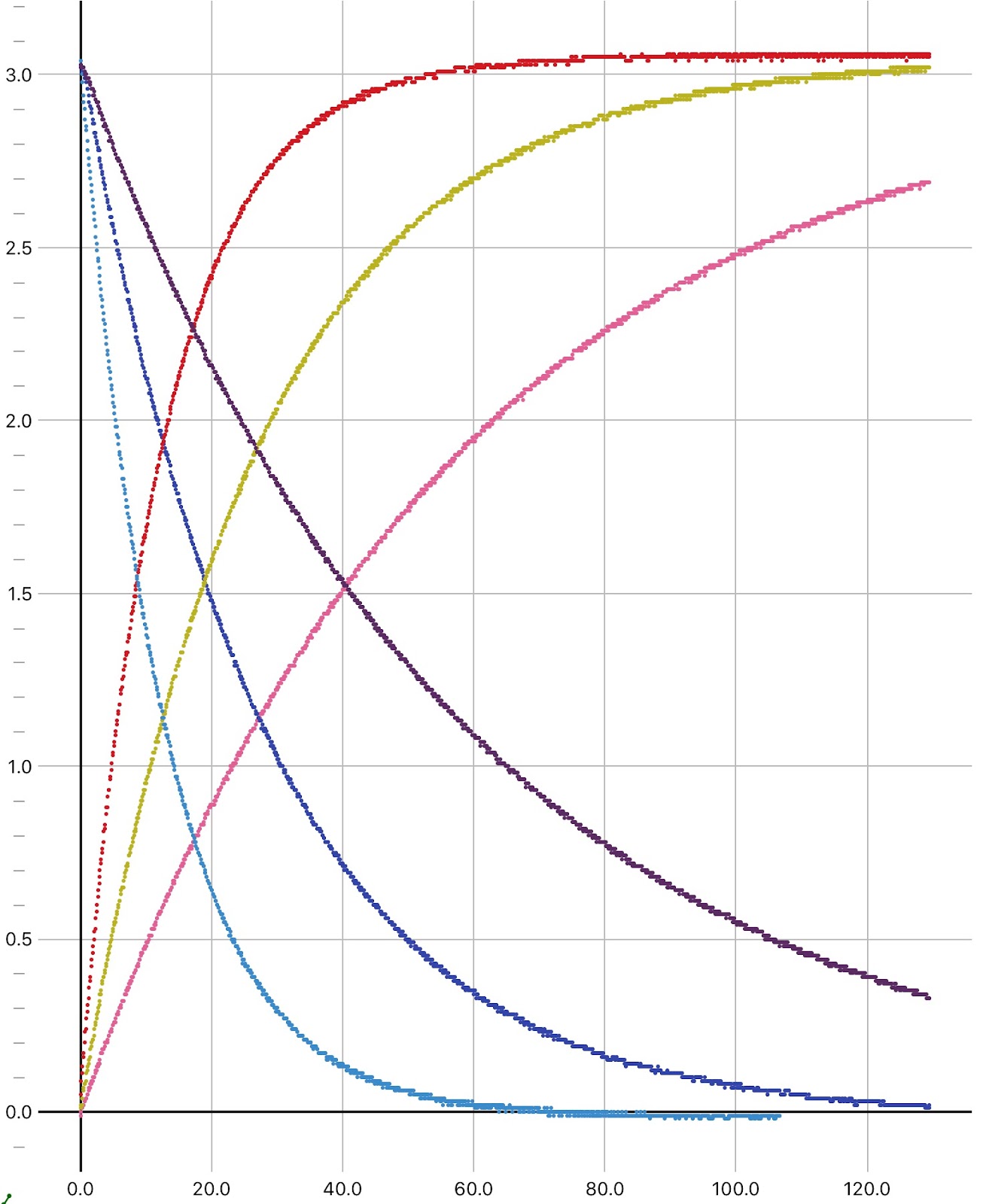
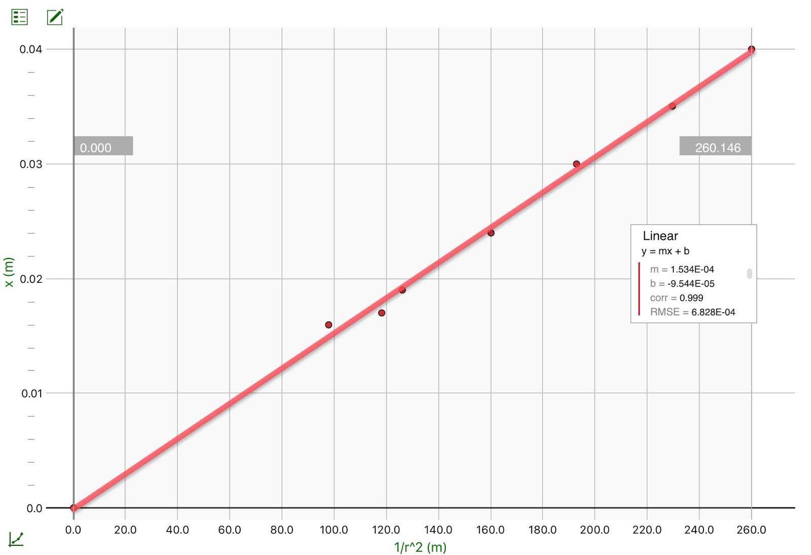
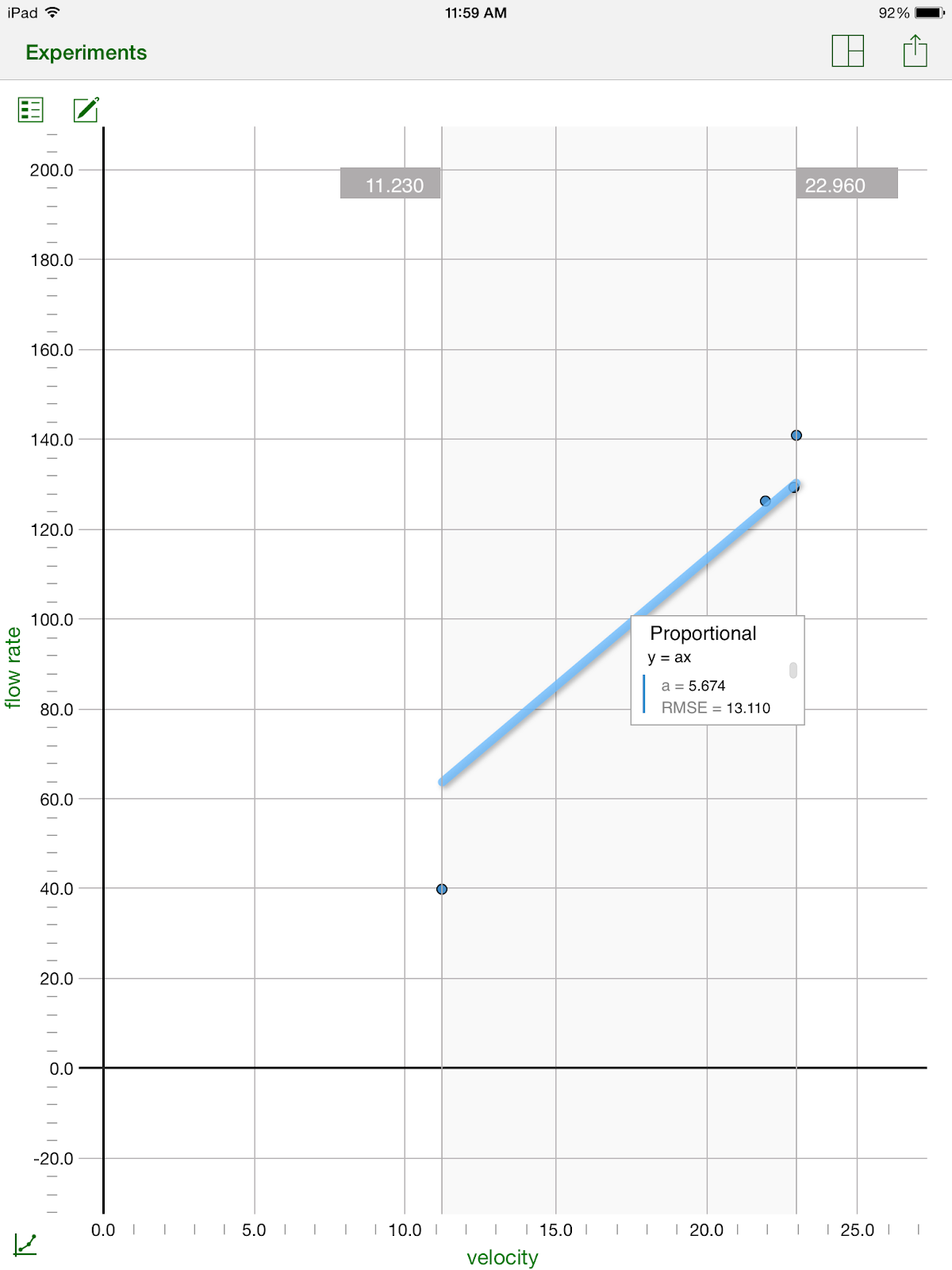
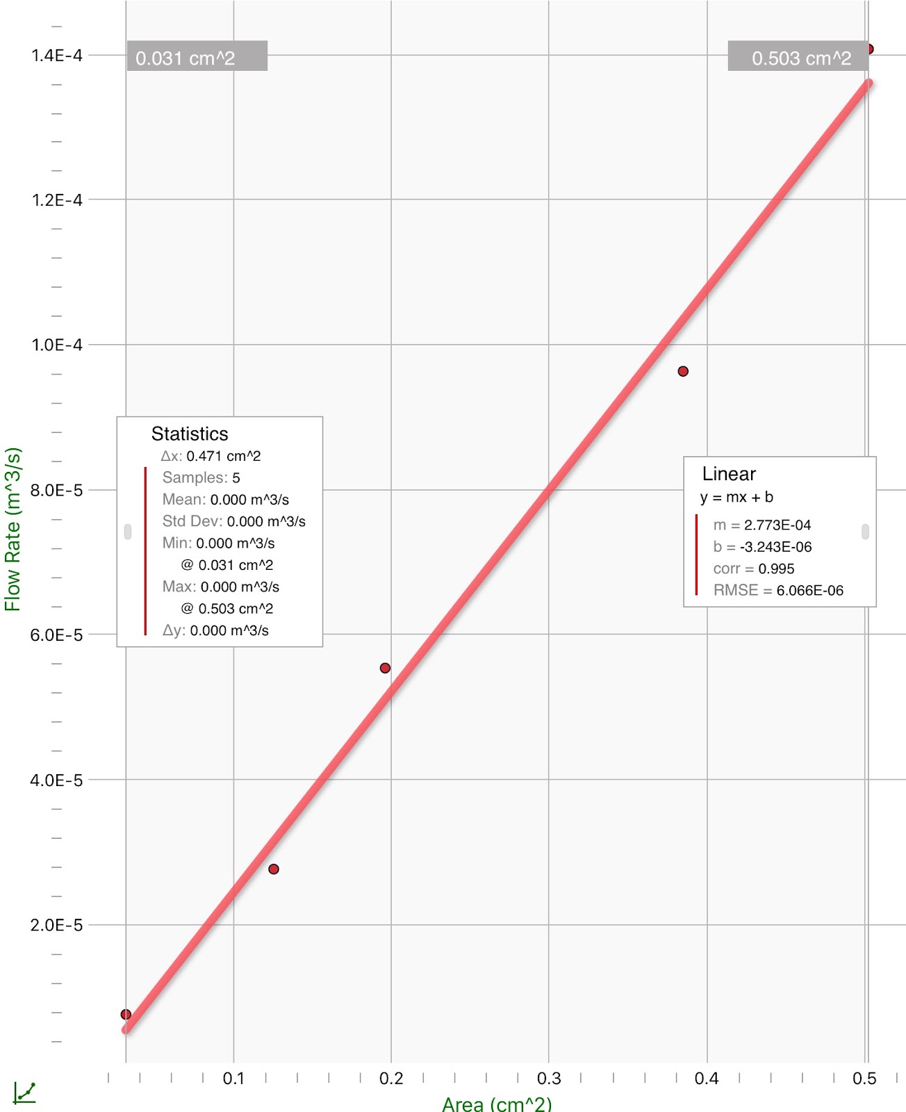
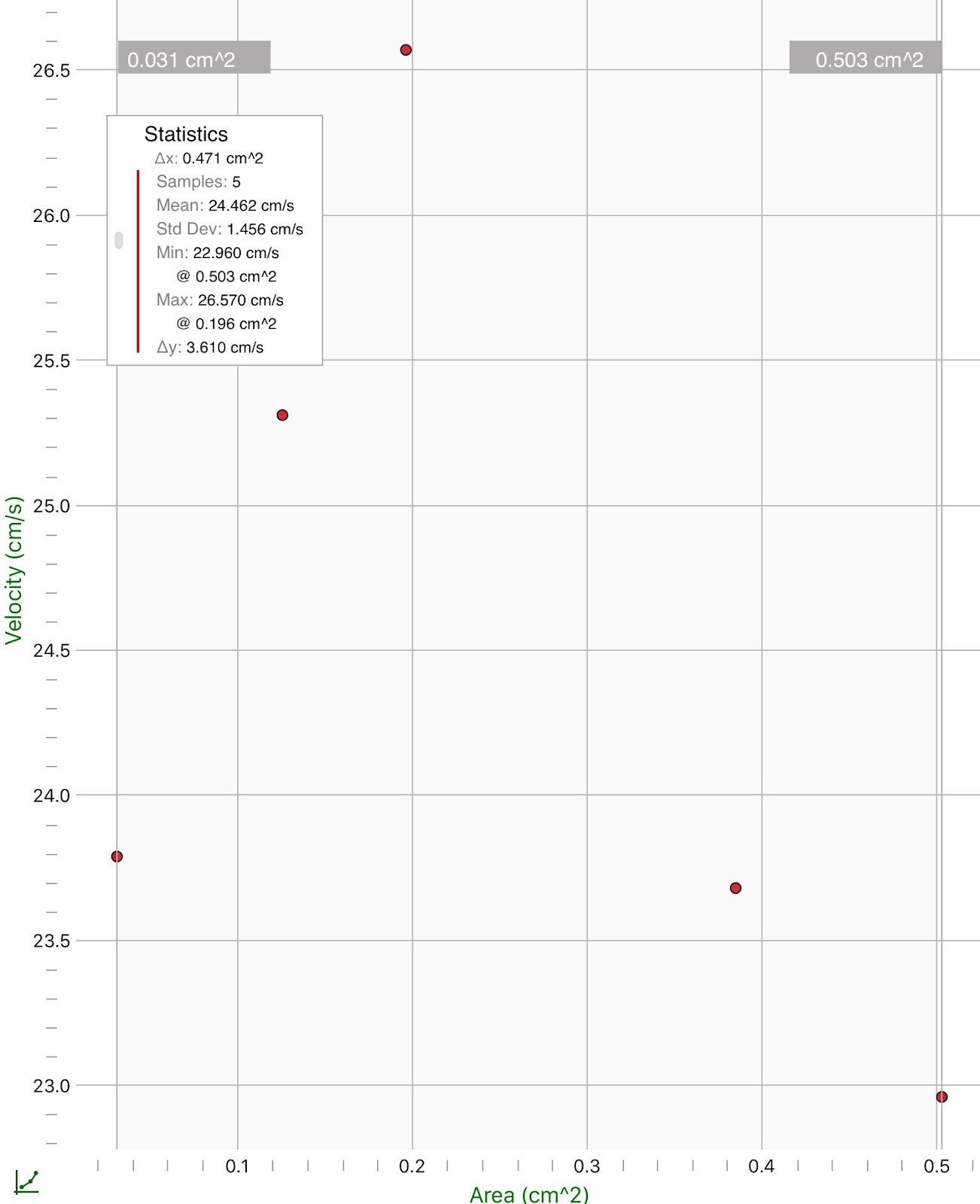
Graphs:

Energy vs. Frequency

Conclusion:

In the first trial the independent variable was photon density and the dependent variable was current. In the second trial the independent variable was voltage and dependent was current. In the third trial the independent variable was wavelength/frequency and the dependent was Kinetic Energy, which was solved for using the equation UK = (4.063 x 10-15eVs)(f) - 2.828eV, where Planck's constant is equal to the slope. The x intercept shows the minimum amount of frequency needed to expel an electron from the Sodium. The y intercept shows us how much force is needed to eject an electron from the Sodium. The generalized equation we can derive from this data is E= hf - ϕ. The slope (h) represents Planck's constant.  The equation E= hf - ϕ shows that kinetic energy of the photoelectron is equal to Planck's constant (h) multiplied by the light’s frequency minus the y intercept (ϕ). The errors that could have happened during our experiment are limited because we used a computer to compute the data used in our analysis. The only way for error to be possible is if we rounded numbers wrong or if we accidentally plugged numbers wrong into our calculator.

AP Physics 2 Unit 11 Lab

Elisa Alvarado, Sarah Cratem, Ryan Partain, Julia Reidy

Mr. Thomas

AP Physics 2 cmod

1 May 2016

Unit 11 Lab: Standard Model

Objective: To determine the graphical and mathematical relationship between deflection angle, new wavelength, and electron momentum.

Apparatus:

Procedure:

1. Go to the website http://www.kcvs.ca/site/projects/physics_files/compton-scattering/compton-scattering.swf
2. Start the experiment with a photon angle of 1 degree and a wavelength of 50pm
3. Click the start button to shoot the photon at the electron
4. Record the electron angle, final wavelength, and electron momentum
5. Repeat steps 2-4 with the photon angles 10, 30, 60, 90, 120, 150, and 180

Data:

Final Wavelength vs. Photon Angle

This relationship does not create a straight line; take the cosine of the x-axis (photon angle) to linearize the relationship.

Final Wavelength vs. cos(photon angle)

This relationship is linear.

Electron Momentum vs. Photon Angle

To linearize this relationship, multiply the electron momentum by the cosine of the electron angle, and for the x-axis, take the cosine of the photon angle and divide it by the final wavelength.

Momentum x cos(Electron Angle) vs. cos(Photon Angle) / Final Wavelength

This graph provides a linear relationship.

Conclusion:

The independent variable is the photon angle and the dependent variables are final wavelength, electron angle, and electron momentum.

The first graph shows the relationship between final wavelength and photon angle which is not a straight line. Then by changing the angle from θ to cosθ it becomes linear and can be described using the equation represented in the second graph:

Final wavelength=-24.245pm(cosθ)+524.235pm

The third graph shows the relationship between electron momentum and photon angle. To linearize this graph, for the y-axis multiply the electron momentum by the cosine of the electron angle, and for the x-axis, take the cosine of the photon angle and divide it by the final wavelength. This gives you the linear equation represented in the fourth graph:

(Momentum e-)(Cos(θ2))=(-0.709yN(s)(pm))(1/final wavelength)(cos(θ1) +11.414yN(s)

Errors in this experiment are unlikely because we used a computer simulation to collect our data. However, some mistakes could have possibly been made in rounding errors and calculations.

AP Physics 2 Unit 9 Lab

Elisa Alvarado, Sarah Cratem, Ryan Partain, Julia Reidy

Mr. Thomas

AP Physics 2 cmod

1 March 2016

Unit 9: Light Wave Model Lab Report

Objective: To determine the effect of object distance on image distance and height for both red and blue lights.

Apparatus:

Procedure:

1. Set up the blue light in a fixed position on the magnetic board.
2. Place the object 16.5 cm away from the light, and use a marker board to view the image, moving it toward or away from the light as necessary to view the focused image.
3. Record the image distance (distance to the marker board from the light) and image height.
4. Repeat steps 2-3 for object distances of 21 cm, 23 cm, 25 cm, 27 cm, 29 cm, 31 cm, and 39.5 cm.
5. Set up the red light in a fixed position on the magnetic board.
6. Place the object 16.6 cm away from the light, and use a marker board to view the image, moving it toward or away from the light as necessary to view the focused image.
7. Record the image distance (distance to the marker board from the light) and image height.
8. Repeat steps 6-7 for object distances of 17.1 cm, 18.4 cm, 20.3 cm, 22.3 cm, 24.3 cm, 27.2 cm, and 38.6 cm.

Data:

Blue Light:

Image Distance vs. Object Distance

This thth

Th

1/ Image Distance vs. 1/ Object Distance

1/di=-0.954(1/do)+0.059cm

-Image Height/ Object Height vs. Image Distance/ Object Distance

-Hi/ho=0.892(di/do)

Red Light:

Image Distance vs. Object Distance

1/ Image Distance vs. 1/ Object Distance

1/di=-1.106(1/do)+0.066

-Image Height/ Object Height vs. Image Distance/ Object Distance

-Hi/ho=0.968(di/do)

Conclusion: The relationship between the two variables, the image distance and the object distance, was hyperbolic. Some constants in the experiment were the lights used. For example the same exact blue light and same exact red light was used throughout the experiment. The lights were also kept at a fixed position on the magnetic board. The material the light traveled through was constant throughout the experiment as well. The equation we got from our data showed that as di/do increased, hi/ho also increased proportionally. The equation from this data is hi/ho=0.968(di/do). To generalize this even more, you can see that (image height/object height)=0.968(image distance/object distance). The slope that we attained was slightly off because we could not maintain a perfect experiment since the slope was supposed to be a value of 1. Therefore, the general equation we derived from our data was hi/ho=di/do(1)=M. Since the value of the slopes were all around 1, another equation that shows the relationship between focal length (F), object distance (do), and image distance (di). This equation can be generalized to show that 1/F=1/do+1/di. Our data is not exactly correct due to errors during the experiment.  For example, we determined when the image was in focus or out of focus using the human eye and judgement.  This was likely to give us slightly incorrect values for each trial.  We also had to measure a shaky image with a ruler.  The image was shaky because lab members had to hold the light in place while we measured the heights and distances.  Our values could have been slightly off due to the shaking of the lasers.

AP Physics 2 Unit 6 Lab

Elisa Alvarado, Sarah Cratem, Ryan Partain, Julia Reidy

Mr. Thomas

AP Physics 2 cmod

13 December 2015

Unit 6: Charged Particles Flow Model Lab Report

Objective: To determine the mathematical and graphical relationship between electrical potential and time for capacitors being charged and discharged when connected to resistors of varying resistivity in series.

Apparatus:

Procedures:

1. Set up the circuit using the 22,000 ohm resistor
2. Charge the capacitor
3. Discharge the capacitor
4. Switch the 22,000 ohm resistor with the 47,000 ohm resistor
5. Charge the capacitor
6. Discharge the capacitor
7. Switch the 47,000 ohm resistor with the 100,000 ohm resistor
8. Charge the capacitor
9. Discharge the capacitor

Data Tables: https://drive.google.com/a/bishopkennyhs.org/file/d/0B2kSUAkE0NVYNGRXcENwUDFncVU/view?usp=docslist_api

Graphs:

Potential vs. Time

Conclusion: While the capacitors are charging, the potential and time are related by the following equation: Vc=Vsource(1-e^(-t/RC)). The graphical relationship between V and t for charging and discharging is represented by the equation (1-ln(Vc/Vs))=-t/RC. While the capacitors are charging, the potential and time are related by the following equation: Vc=Vsource(1-e^(-t/RC)) which can be converted to ln(1-(Vc/Vs))=-t/RC.  We plotted Vc/Vs for the purpose of finding the slope of the final equation and linearizing the graph. The slope was found by the equation slope=1-ln(Vc/Vs)/r where r=resistance with the units of ohms/s. The resistance of the resistor affects the system by lowering the potential and increasing the time it took the circuit to charge. As the capacitance went up the charge and stored charge also rose. Some error could have occurred through a misreading of the devices, batteries not being completely charged, or small amounts of internal resistance on the circuit. The error could be minimized by making sure all equipment is up to date and read properly and carefully.

AP Physics 2 Unit 4 Lab

Elisa Alvarado, Sarah Cratem, Ryan Partain, Julia Reidy

Mr. Thomas

AP Physics 2 cmod

13 December 2015

Unit 4: Charged Particle Interaction Model Lab Report

Objective: To determine the mathematical and graphical relationship between electrostatic force and distance between a neutral and charged object, and to determine the graphical and mathematical relationship between electric force, distance between a neutral particle and a charged particle (r), and the distance traveled by the neutral particle (x).

Apparatus:

Trig Relationships and Force Diagram:

Procedures:

1. Place physics stand 1 meter apart and place the meter stick on top of the stands. Tape the meter stick to the stands. Apply a charge to one balloon by rubbing it against your hair.
2. Tie the strings to the stands and tie the one balloon to each string
3. Separate the charged balloon from the uncharged one until the uncharged one is unaffected by the charge and is at rest directly between the stands.
4. Bring the charged balloon closer to the neutral balloon until the neutral balloon moves and measure the distance between the two and the distance the uncharged balloon was displaced.
5. Repeat the 4th step 8 times and be sure the same increments are used for each trial. Record the space between each of the balloons and how much each balloon is displaced during each trial.
6. Calculate the electric force using net forces and trigonometry as shown in the diagrams above.

Data Tables:

Graphs:

This shows an inverse relationship between delta x and r. To linearize this graph we must take the inverse squared of the quantity r.

displacement vs. 1/r^2

This graph shows a linear relationship between displacement and 1/r^2, as represented by the equation Δx = (1.53 x 10-4m3)/r2.

This graph shows an inverse relationship between electrostatic force and distance between the two balloons. To linearize this relationship we must take the inverse squared of the quantity r.

This graph demonstrates a linear relationship between electrostatic force and the inverse squared of r, represented by the equation Fe= (7.768x10^-6 Nm^2)(1/r^2).

Conclusion:

Our first graph showed an inversely proportional relationship between the change in position of balloon 2 and the distance between the two balloons. To linear use this graph we took the inverse quaked of the quality r. This left us with the relationship of delta x is proportional to 1/r^2.  Since electric force follows this same relationship, we can infer that Fe is proportional to 1/r^2. To determine the electric force we used the force diagram above. From this force diagram we used trigonometry to find the equation Fe = mgtanθ. When you solve for theta using trigonometry the new finalized equation comes out to be Fe=mgtan(Δx/0.2). M is the mass and g is the gravitational constant. To make a general equation to relate the electrostatic force to 1/r^2 we added in a constant k to represent Coulomb's constant. So that Fe = k/r^2. Since the force and the charges show the same proportional relationship to one another we added in Fe=(kq1q2)/r^2. The slope from out linearized graph gave us the number 7.7e-6Nm^2  which represents the product of Coulomb's constant and the charges. ( 7.7e-6Nm^2 =kq1q2)

Error in this lab could have resulted from human errors from measuring the exact distances the objects moved. There could have also been error with the charge of the balloon being greater or lesser at some time.

AP Physics 2 Unit 3 Lab

Elisa, Sarah, Ryan, Julia

Mr. Thomas

AP Physics 2 cmod

15 September 2015

Unit 3: System of Flowing Particles Model Lab Report

Objective: To determine the effect of volume of a tube on distance and volume of water expelled through different-sized holes.

Apparatus:

Procedures:

1. Connect sections of tube to a height of 153 cm from bottom of tube up to the excess hole.
2. Turn hose on and place in the open top of the tube. Wait for the water to rise to and exit out of the excess tube.
3. Measure the horizontal distance the water exits the horizontal holes in the tube from the base of the tube to the end of each stream.
4. Measure the volume of water expelled from each hole in [] seconds by holding a bucket in each stream for the set time.
5. Repeat this procedure for tube heights of 142 cm, 119 cm, and 57 cm, and when measuring the volume of water expelled in a given time, for [] seconds, [] seconds, and [] seconds, respectively.

Data Tables:

Graphs:

Velocity vs. Height

The relationship between velocity and height creates a curve. To linearize this, the values for velocity must be squared.

Velocity Squared vs. Height

The relationship between velocity squared and height is proportional, described in the equation v^2=4 m^2/(s^2 cm)h. This relationship should, however, be described in the equation v^2= (2g N/m)h, where 2g is the slope.

Flow Rate vs. Height

The graph of flow rate vs. height has a relationship that results in a curve. To linearize that we must square the flow rate.

Flow Rate^2 vs. Height

The graph of flow rate^2 vs. height shows a proportional relationship as described in the equation Iv^2=(121 m^5/s) h.

Flow Rate vs. Velocity

The relationship between flow rate and velocity is proportional, as described in the equation Iv=(5.67 m^2)

Flow Rate vs. Area

The relationship between flow rate and area, when the height of the pipe is 153cm, is linear, as shown by the equation: Iv=2.773E-04 m/s(A) - 3.243E-06 m^3/s.  The slope of this line is velocity.

Velocity vs. Area

As shows by the data, the exit velocity of the water is not affected by the area of the hole.  All of these values were obtained when the height of the pipe was 153cm.

Conclusion:

The relationship between velocity and the height of the pipe is that the higher the height, the greater the velocity becomes. An equation that can be used to describe this is  v^2=2gh. The relationship is between flow rate and velocity is that they are directly related and it follows the equation, I=AV. These graphs show that the velocity of a fluid is dependent on the height of the tube and the area which it travels through. The flow rate depends on the area of the hole that it flows out of. The slope of the velocity squared vs. height graph shows us that the slope should be 2 times the gravitational constant "g". The slope of the flow rate vs. velocity means that the velocity and flow rate are proportional to one another. There are no y intercepts for the graphs because they are proportional. Some errors in this experiment could have been with our trials because we didn't have enough time to do all of the trials we wanted to.  Also, errors could have happened with our measurement of the distance the water sprayed to find the velocity, because it was very hard to tell exactly where the water hit the measuring tape. Another error that could have happened was with the angle we held the pipe up with, it could have been not completely straight up. It is also possible that small amounts of water could have been lost while transferring it from the containers to the beakers or graduated cylinders for measurement. These possibilities may have caused varied results in the experiment.