AP Physics Lab 4

Balanced Forces Particle Model Lab

Tyler Kolby, Gabrielle Murphy, Ryan Partain, Trey Seabrooke

Objective

To determine the mathematical and graphical relationship between the mass of an object and the force of gravity acting upon it.

Picture of Apparatus

Procedure

1. Obtain a balance, a spring scale, a stand, and 22 washers.
2. Set up the stand. Attach the spring scale onto the stand.
3. Measure the mass of two washers on a balance and record in the data table.
4. Place the washers on the metal piece suspended from the hook on the spring scale.
5. Record the force of gravity measured for the washers in the data table.
6. Repeat steps 3-5 ten times, adding two more washers to the previous number of washers and recording the measurements in the data table.

Data

Force of Gravity vs Mass Graph

Analysis and Conclusion

The force of gravity vs mass graph shows that as the masses of the washers increase, the force of gravity also increases. This is a direct, linear relationship between the force of gravity and the masses of the objects. Because of this linear relationship, the general equation y=mx+b can be used. In this experiment, y can be replaced by the force of gravity, FG. Additionally, x can be replaced by the mass, m. The y-intercept, b, would be zero - if there were no mass on the spring scale, the force of gravity acting on that mass is zero. The slope, m, can be calculated from the graph, resulting in: m=9.7N/kg. The mathematical relationship to describe this graph can then be explained through the following equation: FG=(9.7N/kg)m.

The slope of the graph, 9.7N/kg, can be related to Earth’s gravitational force on all objects - for every mass on earth, the gravitational force is the mass multiplied by the constant, 9.7N/kg. Due to errors in the experiment, this slope is slightly off, and the value should be closer to 10N/kg. The slope of the graph represents the strength of the Earth's gravitational force field - the gravitational force for each mass at that point in space. A more generalized equation that can be used to represent this would be FG=gm, where "g" is used to represent the slope and therefore the strength of Earth's gravitational force field - 10N/kg.

Some errors were present during this experiment. Each washer was a different mass; because of this, the addition of washers would not have been in equal increments. The result would be a variation in the data as the masses of the washers increased. Another source of error is that the balance used may not have been the most accurate, so the measurement of the masses could have been a little off. We also might not have had the most accurate scale to hold the washers. We could improve this if we used more accurate materials to measure and washers with more similar masses.

AP Physics Lab 3

Momentum Transfer Model Lab

Katie O'Byrne

Michael O'Connell

Chris Prattos

Ryan Partain

Objective: to determine the graphical and mathematical relationship between the ratio of masses to the ratio of velocities of two carts exploding.

Our group's ratio - 4:2

Materials and diagram:

Track with stoppers

One cart without a spring (508 g)

One cart with a spring (513 g)

4 individual weights (~500 g)

Ruler

Balance

Procedure:

1) place both carts on the track without weights

2) set off the spring with a ruler until you find the position at which they hit the opposite stoppers at the same time

3) Record your starting position (ours was 71 cm)

4) Find and record the displacement between starting and ending position for each cart and find the ratios of cart A's displacement to cart B's displacement (d1,d2)

5) Put one weight on cart A for a ratio of 2:1

6) Repeat Steps 2-4

7) Use additional weights to attain the following approximate ratios of the carts masses while(3:1, 3:2, 4:1, 4:2 and 4:3) , and repeat steps 2-4 for each

         Note~ when attaining the ratios, the masses may not be exactly 2:1, 3:1, ect, find the exact ratios of the masses and record them in the Data Table

8) find the inverses of your previous ratios so as to attain 1:2, 1:3, 2:3, etc. and record the data

Data Analysis:

Conclusion:    

    When we first graphed the data, it formed an inversely proportional relationship. As the mass of the carts increased, the displacement of the carts decreased. in order to linearize the data we took the inverse of the x-axis or mass values. This created a linear line of  which we were able to find the slope. This gave us the equation d1/d2= (0.72) M2/M1. However displacement  can be rewritten as velocity (V1/V2) for both carts traveled their distances in the same amount of time. Also, because one cart’s displacement was negative for it moved in a negative direction the equation must be V1/V2= (-0.72) M2/M1. The slope in this equation represents the amount in which the momentum of the two carts changed when the mass increased.

    In this lab, the data for each ratio came from a different group in the class. This left room for some errors such as each group’s track was a different length, thereby changing the starting and stopping points of the carts. We also could have hit the button that released the spring differently each time, either from an angle or with different force. Repeated trials could have loosened the stoppers by being repeatedly hit by the carts that could lead to slight errors in the displacement measurements.  One more possible source of error could be from slight variations in the starting points of the cars.  It looked the same to the human eye, but it is possible that the starting position changed a little each time we hit the cars.

AP Physics Lab 2

Lab #2

Katie O’Byrne, Michael O’Connell, Chris Prattos, Ryan Partain

Constant Acceleration Particle Model Lab

Objective: To determine the graphical and mathematical relationship between position and clock reading for a ball rolling down an incline.

Materials and Diagram:

-Ramp (with 10 cm increments)

-Stand with ramp attached at hole 12

-Metal Ball

-Photo Gates

-Photo Gate Timer

Procedure:

1) Set up stand and attach ramp at hole 12 from the bottom

2) Place photogate A at 10cm and photogate B at 20cm.

3) Clear all readings on the photogate timer

4)Place metal ball at top of ramp and release

5) Record time in seconds for photogate A, photogate B, and the time it took to get to photogate A to B.

6) Repeat steps 3-5 leaving photogate A at 10 cm and moving photogate b in 10 cm increments

7) On trial 8 skip 90cm and move photogate B to 100 cm for the final trial.

Data:

Table for Velocity-Time Graph

VB=(d/tB)

d=1.90cm

(For the VB and tB quantities, view the graph above)

Data Analysis:

X=(215.40cm/s^2)t^2+(80.544cm/s)t+10.637cm

X=(349.955cm/s^2)t^2+20.705m

V=(425.241cm/s^2)t+89.7cm/s

Conclusion:

1. Describe the motion studied in terms of both position and speed and explain the motion map

which represents the motion. Include qualitative motion map showing velocity and acceleration

vectors.

The position changed at faster rates per second and therefore the motion had increasing velocities. The object traveled a greater distance per second as the ball continued down the ramp. The velocity then increased as shown by the increasing length of the arrows in the motion map. The change in velocity (acceleration) however was constant.as shown by the same sized arrows in the motion map .

2. Explain the relationship between variables seen in the x-t and x-t^2 graphs. Show and explain the equations you developed and include numerical values for your constants.

As the object rolled down the ramp , it  changed positions  at a faster rate per second. This caused the graph to form a quadratic relationship or curve.  The equation for the position time graph  is x=½at^2+ V0t+ Xo.  A represents acceleration, V0 represents the velocity at time zero and X0 represents position where time is zero.  T represents time, while x represents position.  The equation for this graph was  X=(215.40cm/s^2)t^2+(80.544cm/s)t+10.637cm; however, in order to find acceleration one needs to find the slope of the velocity, which is the slope of the position vs time graph. In order to find the slope of the position vs time graph we first had to linearize the data. We did this by squaring the time values  which formed a straight line.  This gave us the equation  x= V0t^2+ X0. The equation for this graph was x= (349.955cm/s^2)t^2+20.705m.

We were able to then find the slope of this line but what it represented wasn’t clear based on the data.  We then created a velocity-time graph in order to understand the meaning of the slope.  The velocity time graph created linear line showing that the velocity was increasing steadily as the ball rolled down the ramp. The ball was accelerating at a constant rate as it rolled down the length of the ramp.  

3. Explain how you determined the velocity at a given point in order to make the v-t graph. (This

will require a bit of detail.)

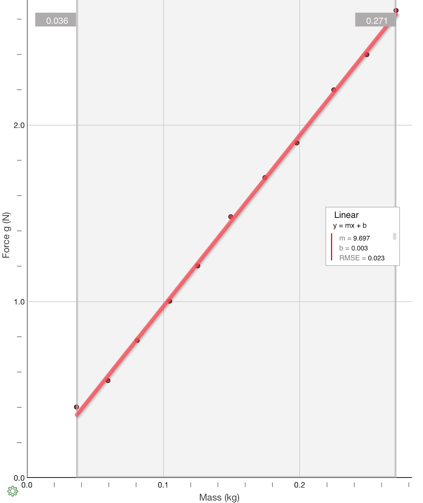
We took the diameter of the ball, 1.90 cm, and divided it by the tB value. the diameter of the ball is the distance it travelled as it rolled. The time it took to travel from the start of gate b to the the end of gate b is the time elapsed)This gave us the velocity at each of the points so we could make the v-t graph.  We plotted the velocity (VB) on the y-axis and the time (tAB) on the x-axis.  The velocity was measured in cm/s, the time was measured in s, and the slope (acceleration) was measured in cm/s^2.

4. Explain the relationship between variables seen in the v-t graph and what this means in terms of the object's motion. Show and explain the equations you developed and include numerical values for your constants.

The relationship is linear (y=mx) or (V=(425.241cm/s^2)t (s))

As the object rolls down the incline the velocity of that object as it enters and exits photo gate b changes as the distance between the ball’s starting point and photogate B increases. This is because the metal ball has a constant acceleration so its velocity is constantly changing. As time goes on the velocity increases linearly as seen from the equation above.

5. Explain the significance of the slope of the v-t graph and provide an interpretation for the slope

without using the word "acceleration." Then provide a formal physics definition of acceleration.

The slope of the v-t graph shows the rate of change in the velocity per second and can theoretically be used to predict the velocity for any given second. Because the slope of the v-t graph is positive instead of zero it means that the object has an increasing change of position per elapsed time meaning that not only is the object changing positions per second but the length of this displacement is also changing.

Acceleration - The rate of change in velocity per unit of time

6. Show and describe how a general velocity equation (consisting entirely of variables) is developed from the v-t graph.

When the v-t graph has been created, an equation can be used as a mathematical model of the graph.  Just like in an x-t graph, the slope is represented by a value.  The slope in a v-t graph is the acceleration.  Instead of using the starting position (like in an x-t graph), the starting velocity is used.  The basic equation for the graph (graph of a line) is y=mx+b.  When using the units and symbols, the final equation becomes V=at+V0.

7. Show and describe how a general position equation (consisting entirely of variables) is developed from the x-t^2graph.

A position equation can be developed from the x-t^2 graph by using the slope of the x-t^2 graph to develop a v-t graph to find the area which is  ∆x which thereby must be equal to ½ of (v+v_0) t. When one makes an a-t graph, one can reason that (v+v_0)=v_0+at+v_0 therefore ∆x=½ (2v_0+at)t which can be simplified to ∆x=v_0t+½ at^2 and then x-x_0= v_0t+½ at^2 into x=½ at^2 + v_0t +x_0.

Some possible sources of error could have been that our photogates could have been imprecise and that we could have dropped the ball at slightly different areas than the exact top of the ramp due to our fingers being slightly sticky from handling our old and sticky photogates. There may also have been slight changes in the air currents in the room as the AC cut on and off but these sources of error probably gave negligible results.

AP Physics 1 Labs

Ryan Partain
Katie O'Byrne, Michael O'Connell, Chris Prattos

Motorized Car Experiment

Materials and Diagram:

• Motorized Car
• Tape Measure (cm)
• Stopwatch (s)

Objective:

To determine the graphical and mathematical relationship between position and clock reading. 

Procedure:

1) Place tape measure on ground and secure it with tape.                   
2) Mark tape at 30cm intervals up until 300cm         
3) Turn on car and release it with the front wheel at zero.
4) Start stopwatch as soon as car is released.
5) Stop stopwatch and pick up the car once the front wheel reaches the thirty centimeter mark.
6) Record time in seconds.
7) Repeat Steps 2-5, increasing the distance to the sixty centimeter mark.
8) Repeat Steps 2-5 for eight more trials, increasing the distance thirty centimeters each time and ending with three-hundred centimeters.

Data:

Data Analysis:

The line of best fit was proportional: X=(V0)t. The y-value was position (cm).  The x-value was time (s).  The slope (V0) was measured in cm/s.

Conclusion:
 
     After testing the experiment, the outcome was that the clock reading was higher when the location of the position of the car increased.  In other words, it took more time for the car to travel a longer distance.  The time and distance traveled shared a direct relationship; as time increased, so did distance. When we graphed the data, the line of best fit was a proportional equation, X=(V0)t.  The slope represented the velocity of the object.  In the final equation, X=(48.603cm/s)t, t represents the x-value (time), m is the slope (velocity), and X represents the y-value.
     The data points may deviate from the line of best fit for a few reasons.  For example, the car may have been set at an angle in the trials. The car was missing some plastic and seemed to curve slightly to the left when  moving forward.  The timer also may have been inaccurate to a few tenths of a second which may have skewed our data since the distances were so short. Conclusively, we may have also placed the car at a slightly different starting point than exactly zero which, with small numbers, could have made quite a few changes in our data along with us failing to react at the exact time to stop the stopwatch at the appropriate interval. However, because all the results were close to the line of best fit, the few errors that did occur were not detrimental to the experiment.