Sunday, March 1, 2015

AP Physics Lab 9

Ryan Partain, Tyler Kolby, Daniel Hanna, Trey Seabrooke

Oscillating Particle Lab

Objective: To determine the graphical and mathematical relationships among mass, amplitude, spring constant, and period for a bouncing mass hanging by a spring.

Picture of Apparatus:
Lab 9 Apparatus.jpg

Materials:
  • Spring
  • Stand w/ latch
  • Hanging mass
  • 10 Washers
  • Timer
  • Ruler
  • Electronic Balance

Procedure:
Obtain all materials listed above and set up the materials to resemble the picture of the apparatus above.
Begin data collection for the various quantities listed in the objective.
To determine force vs. height, set up the apparatus like pictured, and allow the hanging mass to hang freely without oscillation. Record the distance the spring is stretched. Repeat this for 8-10 different masses.
To determine mass vs. period, set up the apparatus like pictures, and allow the hanging mass to hang freely, then stretch the spring to allow oscillation. Keep the amplitude, or distance you stretch the spring constant and record the time of 10 oscillations to find the period for 8-10 different masses.
To determine amplitude vs. period, keep the hanging mass constant. Stretch the spring and record the time for 10 oscillations. Stretch the spring every half centimeter from .5cm to 6cm.
To determine period vs. spring constant, calculate your group's k value from the force vs. height graph and then combine your k with every other group to get the values for the graph.

Data Table:
Lab 9 Data Table.png

Graphs:
Force vs. Height
Force vs. Height.png

Period vs. Mass
Period vs. Mass.png

Period^2 vs. Mass
Period^2 vs. Mass.png

Period vs. Amplitude
Period vs. Amplitude.png

Period vs. Spring Constant
Period vs. Spring Constant.png

Period vs. 1/Spring Constant
Period vs. Spring Constant-1.png

Period^2 vs. 1/Spring Constant
Period^2 vs. Spring Constant-1.png


Conclusion: For the graph of weight vs. extension, the relationship is linear and the slope is the k value or spring constant.
For the graph of period vs. mass, the relationship is parabolic. The period is squared to linearize this graph.
For the graph of period vs. amplitude, there is no relationship.
For the graph of period vs. spring constant, the relationship is inverse. The inverse of the spring constant is taken and the relationship is parabolic. The period is then squared to linearize the graph.
Based on the relationships we see in our graphs, we see the relationship that T(period)=2π(the square root of (m/k))

When experimenting, the timekeeping is a source of error because one person has to communicate to the other that the particle has oscillated ten times (in our case) in order for him to stop the time. Another source of error is that it is difficult to pinpoint exactly when the particle reaches the end of its period making timing more inconsistent and slightly less accurate.Using a motion detector to track the particle would be more effective and accurate in this experiment because it can keep accurate time and also knows exactly when ten periods have elapsed when it's data is graphed.

Monday, February 9, 2015

AP Physics Lab 8

Trey Seabrooke, Ryan Partain, Daniel Hanna, Tyler Kolby

Title: Rotating Bodies Model

Purpose: to determine the graphical and mathematical relationship among net force, mass, distribution of mass and angular acceleration for a rotating pulley.

Procedure:
1. Obtain all necessary equipment to record data for rotating bodies model.
2. Three sets of data will be recorded: changing the mass of the hanging mass while keeping the pulley mass and radius constant, changing the pulley mass while keeping the pulley radius and hanging mass constant, and changing the pulley radius while keeping the hanging mass and pulley mass constant.
3. Change the mass of the hanging mass for eight data points and record the time it takes the hanging mass to reach the ground from the bottom edge of the pulley each time.
4. Change the mass of the pulley for eight data points and record the time it takes each to reach the ground from the bottom edge of the pulley.
5. Change the radius of the pulley for eight data points and record the time it takes each to reach the ground.
6. Convert data to rate units of rad/s^2 for all three data sets.
7. Graph all three sets of data and linearize as needed.

Data Tables:
9.6.png

Graphs:

Angular Acceleration vs. Net Force
9.1.png

Angular Acceleration vs. Mass (swinging)
9.2.png

Angular Acceleration vs. 1/Mass (swinging)
9.3.png

Angular Acceleration vs. Radius
9.4.png

Angular Acceleration vs. 1/Radius^2
9.5.png

Conclusion:
1. A) Angular acceleration versus Fnet is linear. Mass and radius of the pulley are held constant

at: .0241 kg and 11.25 cm respectively.

Angular acceleration versus Mass of pulley is inversely proportional: y vs. 1/x to linearize. Mass

of hanging mass and pulley radius are held constant at: .0908 kg and 11.25 cm respectively.

Angular acceleration versus pulley radius is inversely proportional: y vs. 1/x to parabolic relation:

y vs. 1/r^2 to linearize. Mass of the hanging mass and mass of the pulley are held constant at: .

0908 kg and .1991 kg respectively.

B) Angular acceleration versus Fnet is related by the equation: α=(32.09rad/Ns^2)Fnet + 8.2

rad/s^2.

Angular acceleration versus 1/ mass of pulley is related by the equation: α=(1.02radg/s^2)1/M(s)

+ 10.60radg/s^2.

Angular acceleration versus 1/ pulley radius squared is related by the equation:

α=(827.8radcm^2/s^2)1/radius^2 -24.6radcm^2/s^2.

C) These equations can be generalized by the equation: α=r(pulley)Fnet/kmr^2 or α=torque/

inertia.

2. The Rotating Bodies Model allowed our group to determine the graphical and mathematical

relationship among net force, mass, mass distribution and angular acceleration for a rotating

pulley. This rotational motion relates to Newton's laws of motion in that a force is acting upon the

pulley to cause motion of the hanging mass at certain accelerations. The equation Fnet=ma

developed by Newton is also related through the rotational equivalent: torque=inertia(α).

Thursday, January 15, 2015

AP Physics Lab 7

Daniel Hanna, Tyler Kolby, Trey Seabrooke, Ryan Partain

Central Net Force Model Lab

Objective: To determine the mathematical and graphical relationship among radius, tension, and speed for an object rotating by a spring.

Procedure:
  • Obtain necessary items for lab
  • Measure mass of washers making sure you have ten times the mass of a single washer.
  • Measure string and mark off at any increments ending up with a final distance being ten times as long as the increment.
  • Choose a constant radius to spin apparatus at and increase hanging mass after every trial
  • Take clock reading after 20 rotations for every trial.
  • Record data and graph.
  • Choose constant mass of hanging mass and spin apparatus again changing radius every  trial.
  • Take a clock reading after 20 rotations for every trial.
  • Record data and graph.

Data Table:
image4.png

Graphs:


V vs. r
image5.png

V^2 vs. r
image6.png

V vs. F
image7.png

V^2 vs. F
image8.png

Analysis and Conclusion
1. A)  The original graphical relationship found for the data was quadratic.
B)  We developed our mathematical equation by squaring the velocity (found on our y-axis).
C)  The equation developed from our data is from the y=mx+b equation. For the data in the graph of v^2 as the y values and Force of tension as the x values, we developed the equation v^2=(.284r/m)Fnet. With the v^2 vs. radius graph we developed the equation: v^2=(6.652 Fnet/m)r. The units of these graphs can be related through the equation Fnet (or centripetal acceleration)= v^2/r.
D) the generalized equation for the experiment is Fnet=v^2/r.
2.      Centripetal force is the force acting upon an object when the object is moving in a circular, continuous direction. The force is directed towards the center of the fixture of the object or the center of the system. For this lab, the centripetal force is directed towards the hand of the student that was holding the tube on the string while the string with a rubber stopper was swinging in a circular, rotational motion around the hand of the student. The equation for centripetal force is as follows:  Ac= m(v)^2/ r, or the centripetal acceleration is equal to mass times the velocity squared, all over the radius.
       According to Newton's laws of motion, if the forces acting upon an object are balanced, then the object in motion will continue in motion in a linear path. For an object traveling in a circular path, because the acceleration is constantly changing direction, the forces acting upon the object are unbalanced. This allows the object to continue motion in an ever changing directional state.
3.      The errors in this experiment were most likely the clock management, the system in place was one student watching the student swinging the weights in the circular motion. The student watching would call "time" when the other student started swinging, this indicated a third student to start a timer. When the first student counts that the second student has swung the rope 20 times in a row, he says "time" again. Because their is no possible way to count for the elapsed time between between when one student notices the 20th spin has swung by, and motioning time is to be stopped, this is the flaw in the experiment.

        If the students were to repeat the experiment, the student who was watching and counting the swings of the rope should have their finger readily placed on the timing button to cut down elapsed time and to cut out the middle man as well in this process. All though they limit student participation, the error has been reduced.

Wednesday, December 10, 2014

AP Physics Lab 6

Gabrielle Murphy (insertion of graphs, objective, creation and insertion of data table, deformation vs. height in conclusion, quantitative models in conclusion, force vs. spring deformation in conclusion), Ryan Partain (creation of graphs, sources of error, beginning of deformation vs. speed in conclusion, force vs. spring deformation in conclusion), Trey Seabrooke (procedure), Tyler Kolby

Objective:
To determine the mathematical and graphical relationship between the distance the spring is compressed (deformation of the spring) and the force of the spring, the maximum velocity, and the maximum height.

Procedure:
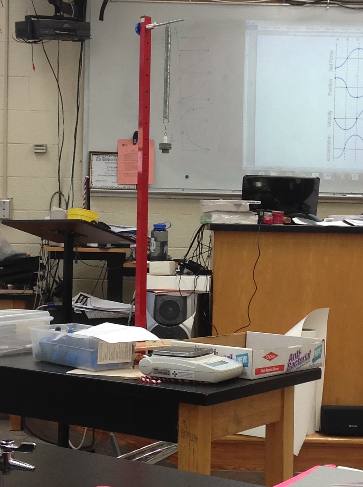
1. Set up an apparatus including: a track(angled 1.2° up from parallel to the ground), a cart, a spring, a force probe attached to the spring, and a motion detector.
2. Place the spring where the track forms the angle with the horizontal. Attach the force probe to the spring.
3. Carefully rest the cart on the spring, with 0 compression of the spring. This is the starting position.
4. Start the motion detector.
5. Compress the spring by pushing the cart against it.
6. Release the cart and record data gathered by the force probe and the motion detector.
7. Repeat steps 3-6 with decreasing compression (less force applied to cart) of the spring each successive time until enough data is collected for the experiment to be valid.
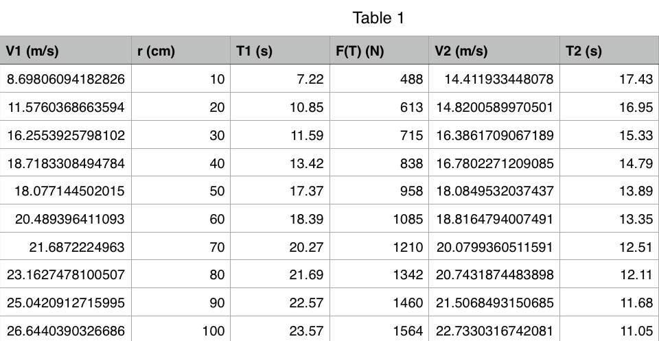
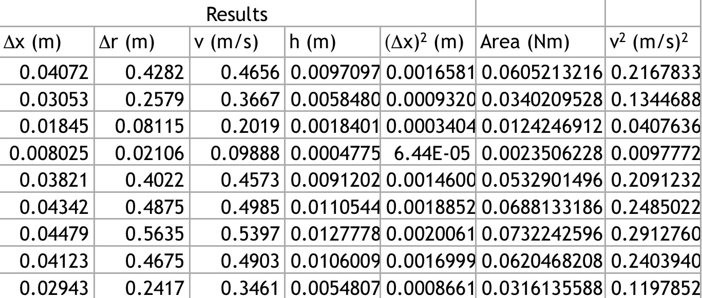
Data Table:

Figure 1
IMG_0470.PNG


Graphs:
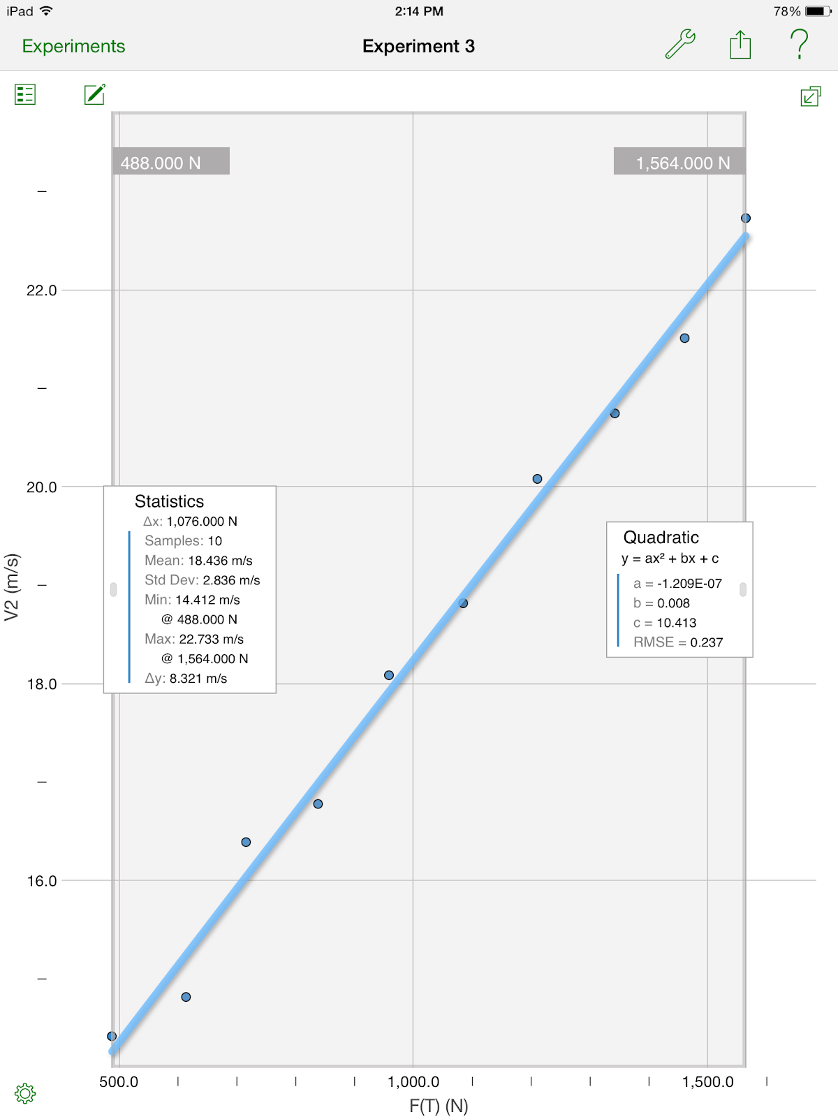
Force vs Deformation (Figure 2)
IMG_0343.PNG

Position (r)vs Time (Figure 3)

IMG_0337.PNG
Time (s)
Velocity vs Time (Figure 4)IMG_0341.PNG


Height vs Deformation (Figure 5)
IMG_0344.PNG

Height vs Area (Figure 6)
IMG_0345.PNG

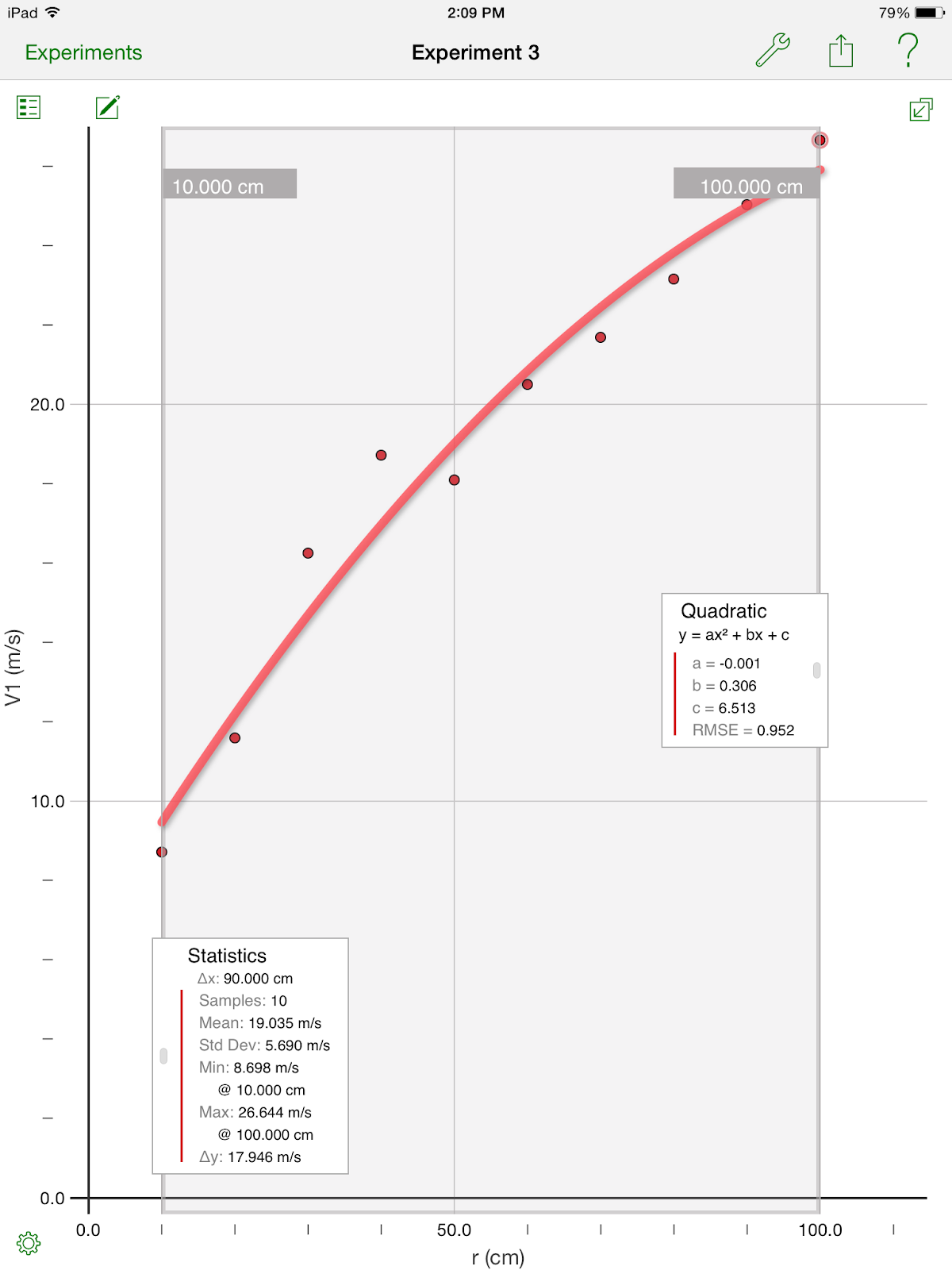
Velocity vs Deformation (Figure 7)
IMG_0375.PNG

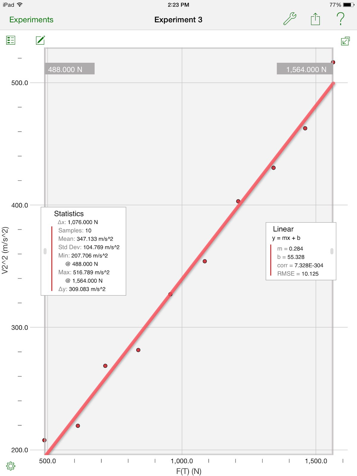
Velocity^2 vs Area (Figure 8)

IMG_0348.PNG

Conclusion:

DEFORMATION VS FORCE

In this experiment, the force exerted on the spring was measured using a force probe attached to the spring. The force required to compress the spring, measured by the force probe, is directly proportional to the distance the spring was compressed, x.  In other terms, the force and spring deformation are directly proportional (as force increases, the spring deformation increases in the opposite direction). Because force and spring deformation are directly proportional, the graph is linear (Fig. 2) and it is in Quadrant II. The slope can be found by the force divided by the spring deformation (N/m). The slope of this graph, represented by the letter k, is the spring constant. The equation created by the force vs spring deformation graph is F=k(x) where k represents the “stiffness” of the spring, or how much the spring resists deformation by a force exerted on it.

The area of the graph can found by multiplying F and x. Because the graph makes a triangle, the area of a triangle equation can be used:

A=(½)bh

where b is substituted by xand h is substituted by F. It can be represented by the equation:

A=(½)xF

Because F= k(x), F can be substituted by k(x) in the area equation. The new equation becomes

A=(½)k(x)^2

This area represents the force that the spring exerts on the cart (the system) that causes the displacement of the cart, which is the work done on the system by the spring. When the system does not include the spring, the equation is

W=(½)k(x)^2

In a system that includes the spring, the energy in the spring is called elastic energy, or U(el). The general equation becomes

U(el)= (½)k(x)^2

DEFORMATION VS HEIGHT

The Position vs Time graph (Fig. 3) can be used to find the relationship between spring deformation (dependent variable) and the maximum height the cart reached as a result (independent variable). Because the track was at an angle, the distance the cart travels on the track, r, can be broken down into two components: xand y where x is the horizontal distance and y is the vertical distance. x, the change in the horizontal, is also the deformation of the spring because it is the horizontal distance the cart and the spring moved when the spring was compressed. x can be found using the minimum value of the Position vs Time graph (Fig. 3) since the cart moves backwards and reaches its minimum position when the spring is at its maximum compression. r is the maximum value of the graph (Fig. 3) because it is the greatest distance traveled by the cart on the track and where it reaches its maximum position. Because the track formed an angle with the horizontal, y, the maximum height, can be found using trigonometry:

h= r(sin)

where =1.2° and r is the maximum of the Position vs Time graph:

h(max)=(0.242 m)(sin 1.2°)= 0.0051 m

The values for h found using the general equation h=r(sin 1.2°) can be graphed in terms of spring deformation,  x to create the Height vs Deformation graph. This would produce a parabolic graphical relationship, as seen in the Height vs Deformation graph (Figure 5). The graph can be linearized by squaring the x-axis - x. The equation for this relationship is

h=NUMBERS(x)^2

The slope of the linearized graph of deformation vs height does not shed light on its relationship since there is no constant in the experiment that can be applied to the slope. Looking at the linearized graph, the height is quadrupled because xis squared. This can be compared to the Force vs Deformation graph (Fig. 2), since xis also a variable in that graph. When xis squared in the Force vs Deformation graph (Fig.2), force becomes squared (because of its linear relationship) and the area under that graph is quadrupled. The two variables affected by the squaring of xthe same way are then be compared to each other to see if there is a meaningful relationship between them: height and the area under the Force vs Deformation graph, or the work done on the system.

To compare Height vs Work,

This new relationship shows that deformation of the spring, which has a direct relationship with how much work the spring does on the cart, will affect the maximum height of the cart.

DEFORMATION VS SPEED

The Velocity vs Time graph (Fig. 3) can be used to find the relationship between spring deformation and the speed the cart traveled during the experiment.  The initial negative velocity on the graph represents when the car was being pushed into the spring, compressing it.  The sudden jump in the velocity is when the car was released from the spring, and it quickly reached its maximum velocity.  Since the track was at a 1.2° angle, the cart slowed as it progressed up the ramp.  The cart eventually reached a velocity of 0 m/s and then started traveling backwards with a negative velocity.  In this experiment, the force of the spring decreased with each trial.  This is the dependent variable, and it caused the velocity to change as a result.  This causes the velocity to be the independent variable.  These results were impacted by the shape of the ramp as well.  Because the ramp was tilted at a 1.2° angle, it caused the cart to slow as time progressed.  The acceleration was in the negative direction because of the Earth’s gravity.  The forces acting on the cart were unbalanced, and gravity was the strongest, pulling the cart down.  This caused the velocity to decrease, reach zero, and then increase in the negative direction as time progressed.
The equation derived from this graph (Fig. 3) is V(max)=

EQUATION MODELS

W=Fx
U(el)=(½)k(x)^2
U(g)=mgh
U(k)=(½)mv^2


SOURCES OF ERROR

During this experiment, many machines were used, and it relied less on human actions.  This reduces the possibilities of errors in the experiment, but there are still possible sources present.  The spring could have been compressed too much or not enough during the experiment.  This would cause inaccurate readings on the force probe, which would lead to errors throughout the experiment.  Since the distance the cart traveled was dependent on the distance the spring was compressed, this reading would also be inaccurate.  Finally, the different amounts of forces applied to the spring could have been inconsistent.  The force applied to the spring was supposed to decrease steadily and constantly, and it may not have been decreased constantly.  This would be yet another source of error during the experiment.