AP Physics 2 Unit 2 Lab

Elisa Alvarado, Sarah Cratem, Ryan Partain, Julia Reidy

Mr. Thomas

AP Physics 2 cmod

9 September 2015

Unit 2: System of Ideal Particles Lab Report

Objective: To determine the effect of pressure of a system on number of particles, volume, and temperature of the system.

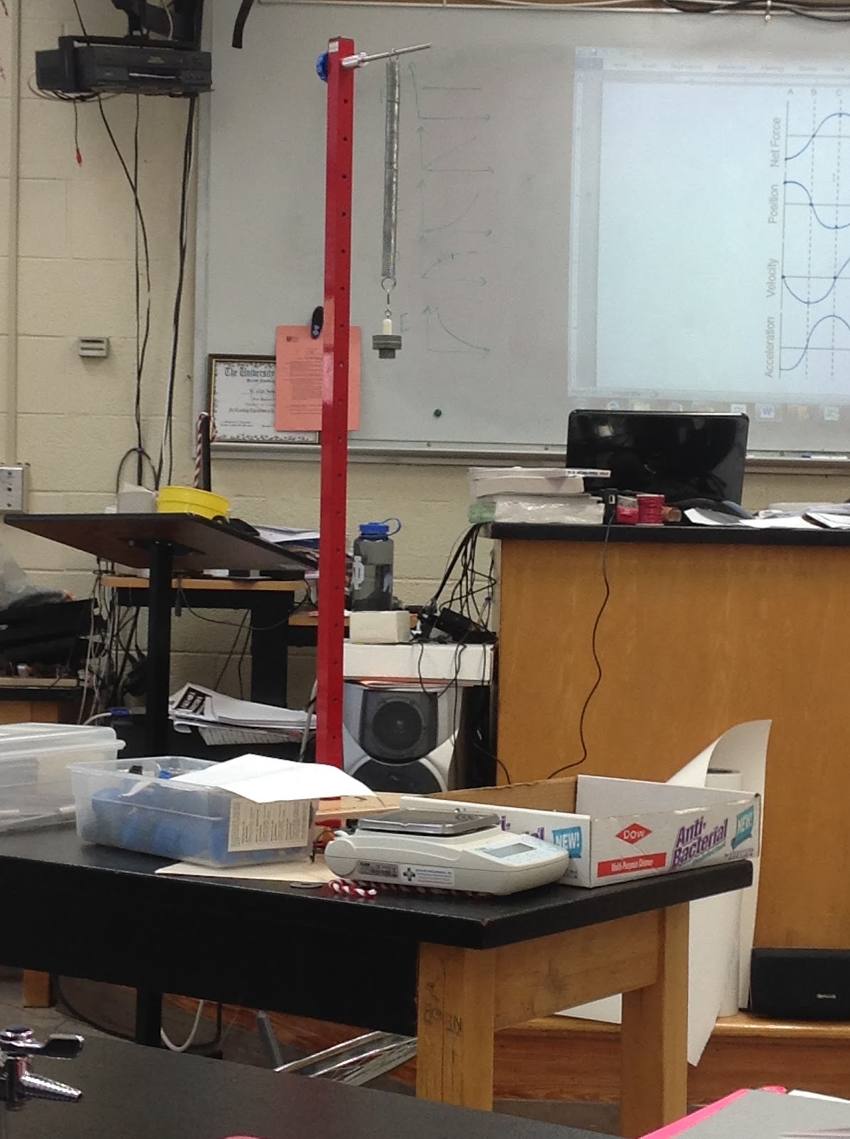
Apparatus:

Procedures:

Pressure vs. Volume:

1. Hook up a syringe to a pressure sensor and take a flask with a stopper attached to it. Attach one hole to the pressure sensor and keep the other end open to be able to open and close it.
2. Fill the syringe up halfway and fill the container and inject the syringe directly into the container.

Pressure vs. Number of Particles:

1. Fill the container up to 20 mL.
2. Open the valve.
3. Fill up syringe halfway. Empty the syringe into the container.
4. Close the valve.
5. Repeat steps 2-4.

Pressure vs. Temperature:

1. Start with close to boiling water.
2. Place the flask and thermometer in a water bath, making sure the water is close to boiling point.
3. Put the magnetic stirrer at bottom of water bath.
4. Submerge the flask in water with the magnet spinning and leave it until it hits equilibrium.
5. Measure the temperature of the water bath.
6. Connect a single-hole stopper to a pressure sensor and measure the pressure.
7. Place small handfuls of ice into water bath and wait until it hits equilibrium.
8. Measure the temperature of the water bath.
9. Repeat steps 2-8.

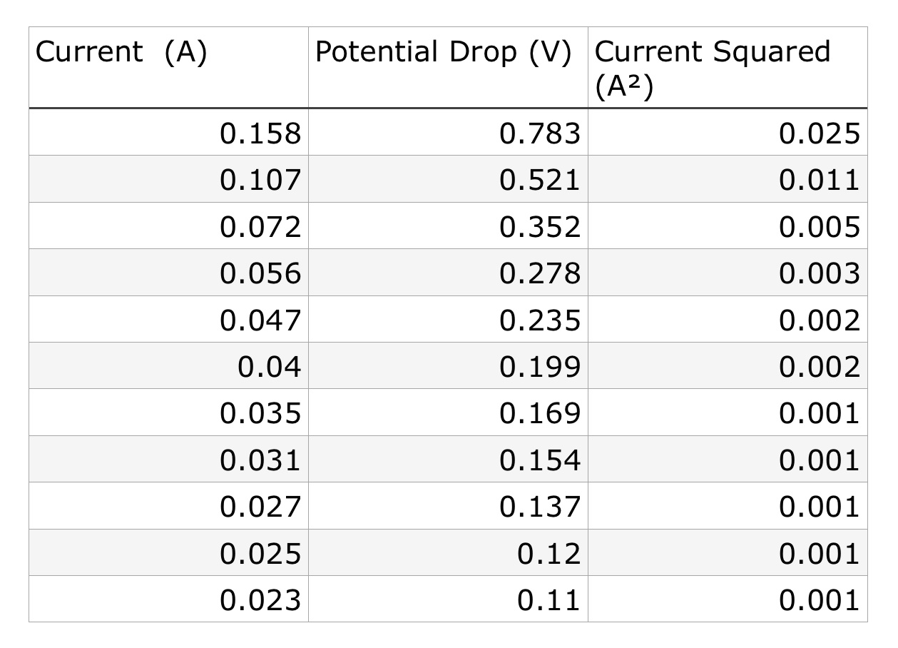
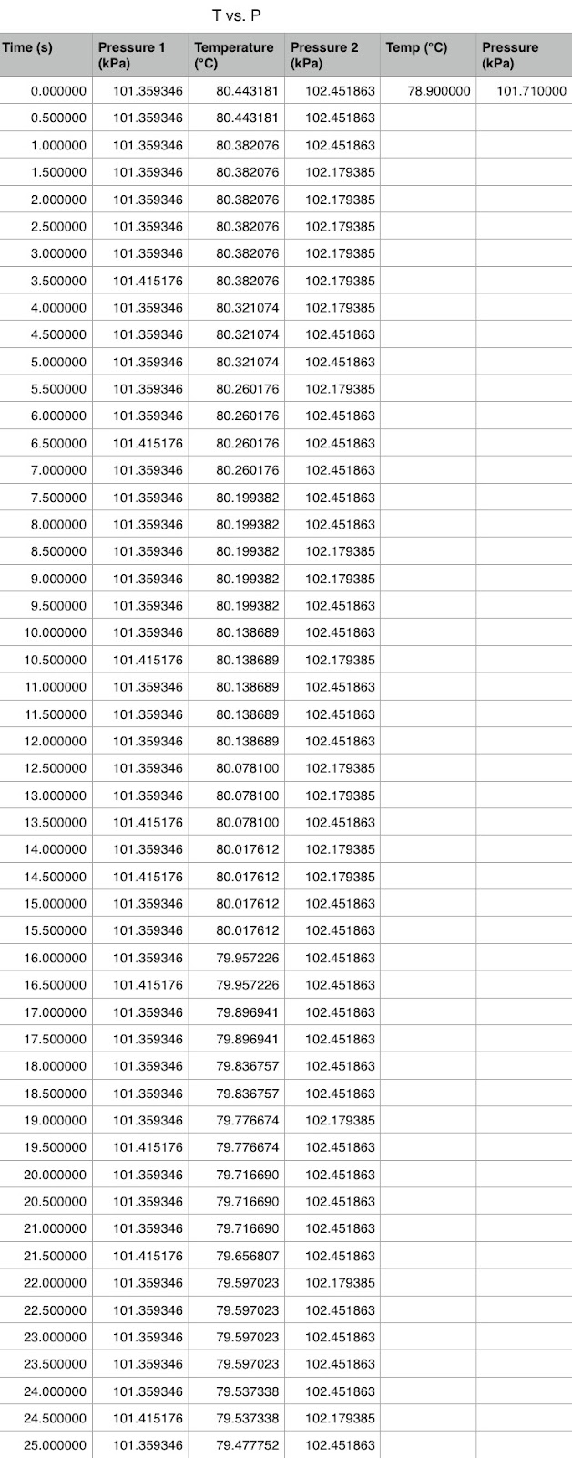
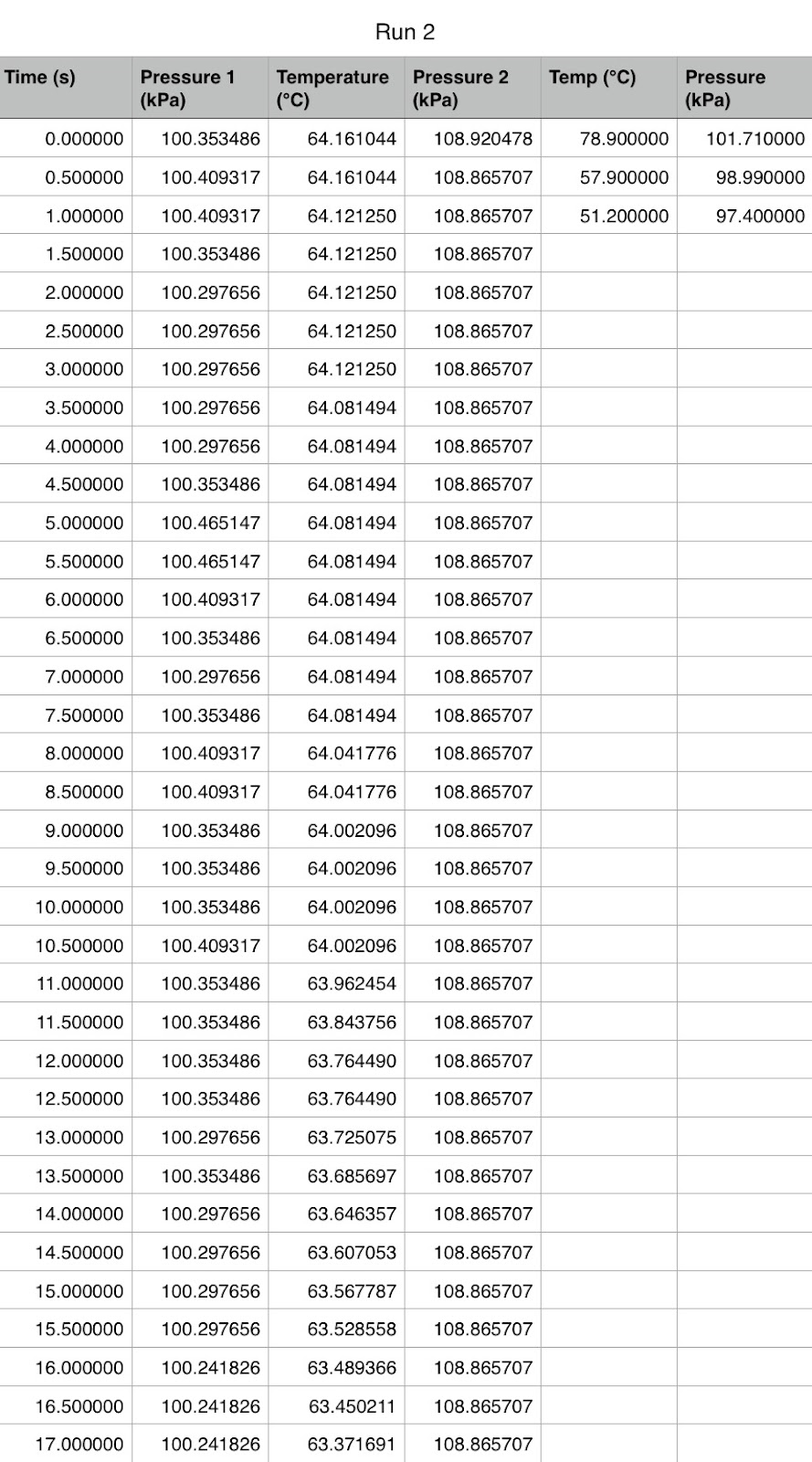
Data Tables:

Graphs:

Number=(5.577kPa/#)(pressure)-(569.017)

Temperature=(4.681kPa/°C)(pressure)-(401.957°C)

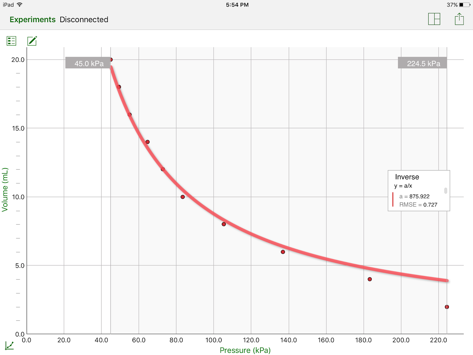
Volume=(875.922mL/kPa)/pressure

Conclusion:

Pressure and volume are inversely related and their relationship can be described in this experiment with the equation Volume=(875.922mL/kPa)/pressure. This forms an inverse graph. Temperature and pressure are directly related and their relationship in this experiment can be described with the equation Temperature=(4.681kPa/°C)(pressure)-(401.957°C). This creates a positive linear graph. Number and pressure are also directly related and can be described with the equation Number=(5.577kPa/#)(pressure)-(569.017) in this experiment.  This also creates a positive linear graph. All of the relationships can be described together with the equation PV=nRT, where volume is measured in liters, pressure is measured in atmospheres, n is the number of moles, the temperature is measured in Kelvin, and R is a constant.  This equation can also be written in another form to work with different units (Pascals for pressure, cubic meters for volume, particles rather than moles, and a different constant, k): PV=NkT.

AP Physics Lab 11

Electrically Charged Particle Model Lab

Brooke Miller, Gabrielle Murphy, Katie O'Byrne, Ryan Partain

Objective: To find the graphical and mathematical relationship between potential and current in a light bulb and two different colored resistors.

Apparatus

Materials:

Battery
Lightbulb
Switch
Dimmer Switch
Resistors (Blue and Green)

Multimeter

Procedure:

1. Create a circuit on the board with the battery, switch, dimmer switch, and bulb connected by wires. Put the dimmer switch on the highest setting.

2. Open the switch to break the circuit. Measure the current across the open switch using the multimeter.
3. Close the switch to close the circuit.
4. Measure the potential drop across the light bulb using the multimeter.
5. Turn the dial on the dimmer switch to the second highest setting and repeat steps 2-4.
6. Repeat steps 2-4 with all the spots on the dial.
7. Take out the bulb and replace it with the green wire (resistor).
8. Repeat steps 2-6 with the green wire.
9. Take out the green wire and replace it with the blue wire (resistor).

10. Repeat steps 2-6 with the blue wire.

Data

Circuit with Light Bulb

Circuit with Green Resistor

Circuit with Blue Resistor

Data Analysis

Lightbulb

Lightbulb Linearized

V=(49.71 V/A2) I2

Blue Wire

V= (9.837 V/A) I

Green Wire

V= (4.937 V/A) I

Conclusion

With the light bulb in the circuit, the potential vs. current graph formed produces a parabolic shape. In order to linearize the data we squared the current. The line gave us the equation V= (49.71 V/A2) I2 where V is potential drop, I is current and the y-intercept is where the current equals zero but is close enough to zero that it is negligible. The slope of the graph represents how difficult it is for the current to move through the circuit, or the resistance present within the circuit.

With the different resistors in the circuit, the potential versus current graphs produce a straight line. As with the experiment with the light bulb, the slope of the line represents the resistance of the wire. The difference between the green and blue resistors were their slopes, or the resistance within the  system; the green wire had a resistance of 5 ohms or (V/A) and the blue wire had a resistance of 10 ohms. This gives us the equations V=(4.937 V/A) I and V= (9.837 V/A) I respectively.

The general equation found for both the blue and green wires is V=IR, where V is the potential drop, I is the current, and R, the slope, is the resistance.

The blue and green resistors have a linear relationship between voltage and current. The graph of the voltage vs current in the light bulb forms a parabolic shape with a changing slope. This difference between the slopes of the green and blue wires and a light bulb because a light bulb is not a “fixed resistor.” While the currents flowing through the systems in each trial are similar throughout all three experiments and the battery is the same, the resistance changes in each trial of each experiment depending on the dimmer switch, which adds resistance. When fixed resistors such as the wires are part of the circuit, the resistance of the wires don’t change even when resistance is changed with the dimmer switch.

Some sources of error could have been that the resistor did not function as well as planned and it had a larger percent error than predicted. The multimeter used also might have been slightly inaccurate and measured incorrect numbers. Energy might have been taken out of the system through heat. The voltage is also slightly lower than expected because potential is lost in the movement across the wires and as the battery continues to power the circuit.

AP Physics Lab 10

Ryan Partain, Trey Seabrooke, Tyler Kolby, Daniel Hanna

Mechanical Wave Model Lab

Objective: to determine the graphical and mathematical relationship between velocity and amplitude, velocity and length of the pulse, velocity and distance, and velocity and force.

Picture of Apparatus:

Materials:

• Distance measurement device
• Spring of length greater than ~1 meter
• Timer
• Force measuring device

Procedure:

To begin, obtain all materials listed above. Lay the spring flat on the ground. Straighten the spring but do not stretch the spring, and record the length of the spring in a straight line.

First record data for the relationship of velocity vs. amplitude. Position the spring at a slightly stretched position and record the length. Two group members are holding the stretched spring at their fixed positions. One group member places his or her foot next to the spring ~1 foot from their end of the spring. The portion of the spring in between the group members foot and the fixed end will now be used to create the amplitude for the pulse. Keep the foot at the same position and change the distance you pull the middle portion of the spring. Record the time it takes for the pulse to go to the other end and return.

Next record data for velocity vs. pulse length. The same setup is used as previously. For this experiment, keep the amplitude constant and move the group members foot at various distances. Record the distances and corresponding time for the pulse to return.

Next, to record velocity vs. distance hold the spring length constant and setup the same as before. Instead of timing the pulse from start to return, now time the pulse from start to half length, start to full length, start to full and one half length, and start two two full lengths to record any change in velocity.

Finally use a force measuring device to determine the force on the spring by the fixed end. Move the spring to get various force values and record the time for the pulse from start to return to determine velocity for each value. Keep the amplitude and pulse length constant.

Data Table:

Graphs:

Velocity vs. Amplitude

Velocity vs. Pulse Length

Velocity vs. Distance

Velocity vs. Force

Conclusion: (no relationship in any except V vs. F.  Despite what appears to be a linear relationship, the data set accidentally followed that general trend, but the numbers were scattered.  Due to experimental error, the data appears to have a relationship despite having none)

In the graph of V vs. F, the relationship is parabolic; therefore V is squared to linearize making the graph V^2 vs. F. Based on this graph we see the relationship V^2=( m/kg)F.

Sources of error include difficulty in pinpointing the exact time one wavelength has traveled the entire length of the spring, and difficulty in keeping the spring in the exact same position throughout the experimental trials. The procedure could be improved if there were more stable fixed positions at the ends of the spring. It could also be improved if the pulses were more accurately recorded. For example, using ones foot works but contributes in error of the experiment due to the width of the foot in contact with the spring.

AP Physics Lab 9

Ryan Partain, Tyler Kolby, Daniel Hanna, Trey Seabrooke

Oscillating Particle Lab

Objective: To determine the graphical and mathematical relationships among mass, amplitude, spring constant, and period for a bouncing mass hanging by a spring.

Picture of Apparatus:

Materials:

• Spring
• Stand w/ latch
• Hanging mass
• 10 Washers
• Timer
• Ruler
• Electronic Balance

Procedure:

Obtain all materials listed above and set up the materials to resemble the picture of the apparatus above.

Begin data collection for the various quantities listed in the objective.

To determine force vs. height, set up the apparatus like pictured, and allow the hanging mass to hang freely without oscillation. Record the distance the spring is stretched. Repeat this for 8-10 different masses.

To determine mass vs. period, set up the apparatus like pictures, and allow the hanging mass to hang freely, then stretch the spring to allow oscillation. Keep the amplitude, or distance you stretch the spring constant and record the time of 10 oscillations to find the period for 8-10 different masses.

To determine amplitude vs. period, keep the hanging mass constant. Stretch the spring and record the time for 10 oscillations. Stretch the spring every half centimeter from .5cm to 6cm.

To determine period vs. spring constant, calculate your group's k value from the force vs. height graph and then combine your k with every other group to get the values for the graph.

Data Table:

Graphs:

Force vs. Height

Period vs. Mass

Period^2 vs. Mass

Period vs. Amplitude

Period vs. Spring Constant

Period vs. 1/Spring Constant

Period^2 vs. 1/Spring Constant

Conclusion: For the graph of weight vs. extension, the relationship is linear and the slope is the k value or spring constant.

For the graph of period vs. mass, the relationship is parabolic. The period is squared to linearize this graph.

For the graph of period vs. amplitude, there is no relationship.

For the graph of period vs. spring constant, the relationship is inverse. The inverse of the spring constant is taken and the relationship is parabolic. The period is then squared to linearize the graph.

Based on the relationships we see in our graphs, we see the relationship that T(period)=2π(the square root of (m/k))

When experimenting, the timekeeping is a source of error because one person has to communicate to the other that the particle has oscillated ten times (in our case) in order for him to stop the time. Another source of error is that it is difficult to pinpoint exactly when the particle reaches the end of its period making timing more inconsistent and slightly less accurate.Using a motion detector to track the particle would be more effective and accurate in this experiment because it can keep accurate time and also knows exactly when ten periods have elapsed when it's data is graphed.

AP Physics Lab 8

Trey Seabrooke, Ryan Partain, Daniel Hanna, Tyler Kolby

Title: Rotating Bodies Model

Purpose: to determine the graphical and mathematical relationship among net force, mass, distribution of mass and angular acceleration for a rotating pulley.

Procedure:

1. Obtain all necessary equipment to record data for rotating bodies model.

2. Three sets of data will be recorded: changing the mass of the hanging mass while keeping the pulley mass and radius constant, changing the pulley mass while keeping the pulley radius and hanging mass constant, and changing the pulley radius while keeping the hanging mass and pulley mass constant.

3. Change the mass of the hanging mass for eight data points and record the time it takes the hanging mass to reach the ground from the bottom edge of the pulley each time.

4. Change the mass of the pulley for eight data points and record the time it takes each to reach the ground from the bottom edge of the pulley.

5. Change the radius of the pulley for eight data points and record the time it takes each to reach the ground.

6. Convert data to rate units of rad/s^2 for all three data sets.

7. Graph all three sets of data and linearize as needed.

Data Tables:

Graphs:

Angular Acceleration vs. Net Force

Angular Acceleration vs. Mass (swinging)

Angular Acceleration vs. 1/Mass (swinging)

Angular Acceleration vs. Radius

Angular Acceleration vs. 1/Radius^2

Conclusion:

1. A) Angular acceleration versus Fnet is linear. Mass and radius of the pulley are held constant

at: .0241 kg and 11.25 cm respectively.

Angular acceleration versus Mass of pulley is inversely proportional: y vs. 1/x to linearize. Mass

of hanging mass and pulley radius are held constant at: .0908 kg and 11.25 cm respectively.

Angular acceleration versus pulley radius is inversely proportional: y vs. 1/x to parabolic relation:

y vs. 1/r^2 to linearize. Mass of the hanging mass and mass of the pulley are held constant at: .

0908 kg and .1991 kg respectively.

B) Angular acceleration versus Fnet is related by the equation: α=(32.09rad/Ns^2)Fnet + 8.2

rad/s^2.

Angular acceleration versus 1/ mass of pulley is related by the equation: α=(1.02radg/s^2)1/M(s)

+ 10.60radg/s^2.

Angular acceleration versus 1/ pulley radius squared is related by the equation:

α=(827.8radcm^2/s^2)1/radius^2 -24.6radcm^2/s^2.

C) These equations can be generalized by the equation: α=r(pulley)Fnet/kmr^2 or α=torque/

inertia.

2. The Rotating Bodies Model allowed our group to determine the graphical and mathematical

relationship among net force, mass, mass distribution and angular acceleration for a rotating

pulley. This rotational motion relates to Newton's laws of motion in that a force is acting upon the

pulley to cause motion of the hanging mass at certain accelerations. The equation Fnet=ma

developed by Newton is also related through the rotational equivalent: torque=inertia(α).